Typical Oscilloscope Voltage Probe Circuits

1. High-impedance passive probe

passive probes have advantages such as low cost, robust mechanical structure, wide dynamic range, and high input resistance, making them widely used in general testing scenarios. The commonly used passive probe is the high-resistance passive probe with attenuation by 10 times, mainly including the probe tip, lossy transmission lines, and compensator. The typical circuit model is shown in Figure 1

Figure 1 10 Typical circuit model of a high-resistance passive probe

The front end of the probe is used to connect the detection point, where the signal end provides a high-resistance resistor Rt to reduce load effects, and is contained in the parasitic capacitor Ct; The ground end is generally a trailing crocodile clip with a parasitic inductance Lg

transmission line is used to provide measurement distance, with a typical length of 1~2m. The transmission line can be equivalent to a lumped component model with distributed parameters such as RLGC. When the terminal impedance does not match, high-frequency signals will resonate. To better suppress this resonance issue, the transmission line can be designed as a lossy type, i.e., with a certain distributed resistance

The compensator is used to match the impedance of the probe and oscilloscope, represented in Figure 2 by an RC series network. According to the compensation attenuator theory, to maintain linear attenuation of the signal over a wide frequency range, the variable capacitance Cc can be adjusted so that the time constants of the input and output networks are equal, i.e

RtCt=Rs(Clt+Cc+Cs).

In this formula, Clt is the total capacitance of the lossy transmission line. According to the working principle of the transmission line, to improve the high-frequency gain of the probe, the variable resistor Rc can be adjusted so that the load impedance approaches the characteristic impedance of the transmission line, i.e

In the formula, Z0 is the transmission line's characteristic impedance; fb is the probe bandwidth

2. active single-ended probe

The front end of the active single-ended probe is equipped with a field-effect transistor, which gives it very small input capacitance but also results in a very limited linear dynamic input range. Additionally, the high cost and fragile mechanical structure of active single-ended probes limit their application range. Figure 2 shows a circuit model of an active single-ended probe with 10x attenuation, mainly consisting of an attenuator, buffer, and lossless transmission line

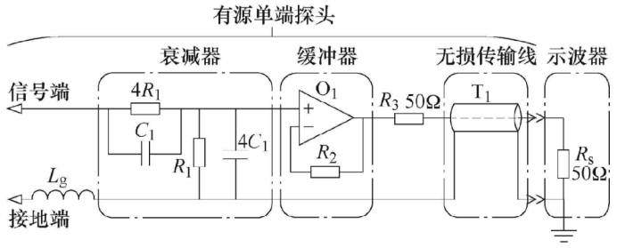
Figure 2 10x attenuation active single-ended probe circuit model

signal is first attenuated 5-fold through an attenuator, then voltage follows via a buffer, and finally transmitted to the oscilloscope via a lossless transmission line. Among them, the buffer has high input impedance and strong output driving capability, isolating the attenuator from the lossless transmission line. This facilitates impedance matching between the input and output terminals, improving signal transmission capability; On the other hand, the attenuator can be placed as close as possible to the test point to reduce uncontrollable parasitic parameters. The characteristic impedance of lossless transmission lines is generally 50Ω. R3 and Rs are matched with the source and load ends respectively to improve signal fidelity and simultaneously attenuate the buffer output signal by 2 times

3. Active differential probe

Active differential probes are mainly used to measure differential signals and can be divided into low-voltage and high-voltage types. Generally, high-voltage differential probes with better versatility are chosen to measure switching power supply signals. Figure 3 shows a classic active high-voltage differential probe circuit model, which mainly includes an attenuator, buffer, differential amplifier, and lossless transmission line. In the figure, Lp+ and Lp- are parasitic inductors at the two signal terminals, respectively

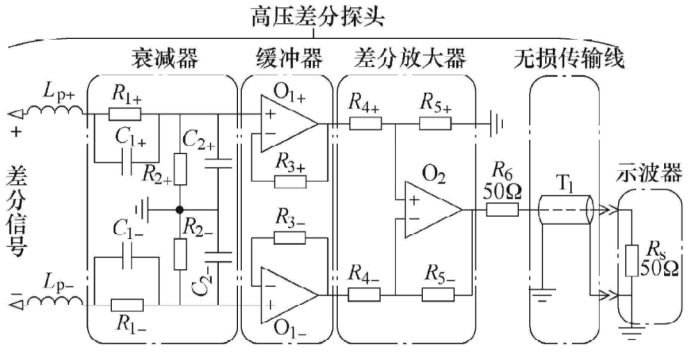
Figure 3 Active high-voltage differential probe circuit model

First, the differential signal is sequentially attenuated and voltage follows through two theoretically identical attenuators and buffers; Then, the differential amplifier converts it into a single-ended ground signal; Finally, it is transmitted to the oscilloscope via a lossless transmission line. The common-mode rejection ratio is an important indicator of a differential probe. The common-mode gain of active differential probes mainly comes from two sources: (1) The incomplete symmetry of resistors, capacitors, buffers, and parasitic parameters in the two differential signal transmission paths; (2) The inherent common-mode gain of the differential amplifier

4. Light isolation probe

The optical isolation probe is also used to measure differential signals. Its block diagram is shown in Figure 4. The probe mainly includes an attenuator, electro-optical-electrical conversion network, lossless transmission line, and oscilloscope connector. The electrical-optical-electrical conversion network serves as the core of the optical isolation probe. Through the electrical-optical converter, optical fiber, optical-electrical converter, and controller, it achieves electrical isolation between the device under test and the oscilloscope, shortening the transmission path of the differential signal. This greatly increases the common-mode rejection ratio of the probe, enabling it to measure differential signals with high bandwidth and high common-mode voltage

Figure 4 Block Diagram of the Principle of an Optically Isolated Probe

Reprinted from Tektronix